Linear Least Square Fitting using GSL
Sometimes for scientific calculation we need to do a least square fitting to a set of data. Depends on the usage, if you need to fit with a line then you need to perform a linear least square fitting, and if you need to fit with a polynomial with higher order, you need to perform non-linear least square fitting.
I have been trying to do this in C++ for a period of time, until I found that I can do it using Gnu Scientific Library. This really helps me a lot and make my job easier.
So, here's how it goes:
1. Make sure Gnu GSL library is configured with your compiler. Please Google it out to find out how.
2. Include the libraries into your program. You might need to visit this site to see how to configure it in Borland C++ Builder 6.
3. Include the header file for fitting into your source code:
#include < gsl/gsl_fit.h >
4. Basically, the function for linear least square fitting is (quoted from this website):
int gsl_fit_linear (const double * x, const size_t xstride, const double * y, const size_t ystride, size_t n, double * c0, double * c1, double * cov00, double * cov01, double * cov11, double * sumsq)
This function computes the best-fit linear regression coefficients (c0,c1) of the model Y = c_0 + c_1 X for the dataset (x, y), two vectors of length n with strides xstride and ystride. The errors on y are assumed unknown so the variance-covariance matrix for the parameters (c0, c1) is estimated from the scatter of the points around the best-fit line and returned via the parameters (cov00, cov01, cov11). The sum of squares of the residuals from the best-fit line is returned in sumsq. Note: the correlation coefficient of the data can be computed using gsl_stats_correlation (see Correlation), it does not depend on the fit.
5. So, we have to use that function. Before that, we should make our data for testing the algorithm. A simple array with random values will be enough, something like this:
spreadData[i] = (double)(rand() % 20 + 1) + (0.5 * i);
6. Then, finally call the line fitting function with the respective input and output arguments:
gsl_fit_linear (dataAxis, 1, spreadData, 1, 100, &c0, &c1, &cov00, &cov01, &cov11, &chisq);
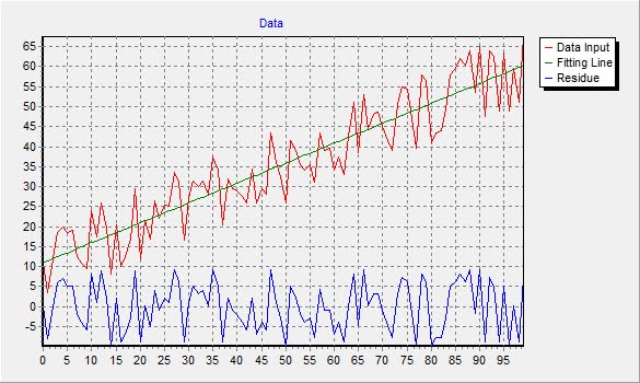
Finally, you can plot the fitted value together with the data. The output that I got is something like this, for this example I plot the residue values together with the data and the line.
Hope it will be useful for you too. Good luck.
Labels: borland c++ builder, coding, gnu scientific library
posted by mario at
12:01 AM
|
0 comments
![]()